Air pollution is a major concern for the modern world.
Prolonged exposure to low quality air resulting from a variety of sources like vehicle emissions, fumes from chemical production, mold spores, and wildfires can lead to several adverse health effects.
Some of the health effects from exposure to poor air quality are irritation of the eyes, nose and throat, shortness of breath, afflictions on the cardiovascular system and even more serious complications after long periods of time.

Apart from the impact that low air quality has on human health, the environmental effects of poor air quality are just as severe. Poor air quality can lead to reduced crop yields as well as increased susceptibility of plants to pests and disease amongst other things.
As such, keeping a close eye on air quality levels is of import to health and the environment.
In this project I'll be exploring the AirQuality Dataset in order to train a set of machine learning (ML) models capable of predicting predicting the concentrations of a variety of pollutants like metal oxides and hydrocarbons.
The data was obtained from the UCI Machine Learning Repository here https://archive.ics.uci.edu/ml/datasets/Air+Quality. This dataset covers sensor collection data on a variety of pollutants spanning from March 2004 to February 2005 (1 year)
You can look at the code heavy version in my Github repository found here or in this post I made here.
Exploratory Data Analysis - How does the data look like?
There was a bit of data clean up that needed to be done prior to doing any of the analysis. If you are interested in the process I carried out
to get it nice and tidy, you can check the Github repository or the post I made. Suffice for it to say that there were null sensor readings
that had to be dealt with, empty columns, redundant data, and improperly formatted time data. I also added columns containing specific time features (i.e.,
Day of The Week, Month, and Hour) to get more detailed information of how the pollutant concentrations behaved in time. The results of my
data clean up can be seen at the end of the pandas_profiling report below.
In addition to ensuring the dataframe had general tidiness, I also noticed that many of the data attributes exhibited skewedness in their distributions. Skewedness in distributions is partially due to the presence of outliers. To deal with this I used the Interquartile Range (IQR) method.
At the end of my data cleanup, I had 6097 measurements left and 13 data features. More specifically, I had 8 features that would end up making it to the subsequent modeling stage.
The features I had to work with from this point on are the following:
- Date (DD/MM/YYYY)
- Month
- Weekday
- Hour
- Carbon Monoxide (CO) Concentration
- Nonmetal Hydorcarbon (NMHC) Concentration
- Nitrogen Monoxide (NOx) Concentration
- Nitrogen Dioxide (NO2) Concentration
- Ozone (O3) Concentration
- Temperature (T)
- Relative Humidity (RH)
- Absolute Humidity (AH)
From these data attributes I decided to generate a pair plot to visualize the correlations and variable relationships a bit better which is shown below.


Beautiful! There's definitely dependencies between some of the variables.
Brief Chemistry Detour
From the pair plot above, it can be seen that the pollutant concentrations are related to one another. They seem to increase together with the exception of the Nitrogen Monoxide readings. The chemist in me finds this pretty interesting! Nitrogen Monoxide is a free radical compound (meaning that it is highly unstable and very reactive). Perhaps it is reacting with one of the other pollutants thus reducing its concentration?
Something else that I noticed from this pairplot is that the Nitrogen Dioxide appears to be correlated with the Absolute Humidity. This is a behavior that none of the other pollutants show. Why?
Combustion engines burn fuels at high temperatures in order to operate. The temperatures of these engines are sufficiently elevated so as to cause Nitrogen and Oxygen molecules to react to form Nitrogen Monoxide:
$$ N_{2}(g) + O_{2}(g) -> 2NO(g) $$Nitrogen Monoxide can then react with Oxygen molecules in the air to form Nitrogen Dioxide:
$$ 2NO(g) + O_{2}(g) -> 2NO_{2}(g) $$As the Nitrogen Dioxide rises, it can interact with Water molecules to form Nitric and Nitrous Acid.
$$ 2NO_{2}(g) + H_{2}O(l) -> HNO_{3}(aq) + HNO_{2}(aq)$$The set of reactions I have described above is how acid rain forms.
Absolute humidity (AH) is the total mass of water vapor present in a given volume or mass of air. It is independent of temperature. As AH increases, it would increase the likelihood for Nitrogen Dioxide to react with water.
Questions to answer
Some of the questions that I want to answer and/or goals I want to accomplish with this project are the following:
- Can we predict the level of a pollutant based on the concentrations of other pollutants?
- At what times/days do pollutant levels maximize/minimize?
- Do all pollutants increase together or do some of them peak/valley at different points?
- Is there any relationship/trend we can infer/deduce with regards to the humidity/temperature from pollutant concentrations?
Time Series of CO Concentration
To figure out when the CO concentration is highest, we can refer to the plots below. The plots below show the CO concentration as a function of unit of time (i.e., year, month, day, hour). These plots can help elucidate the time periods that maximize pollutant concentration.
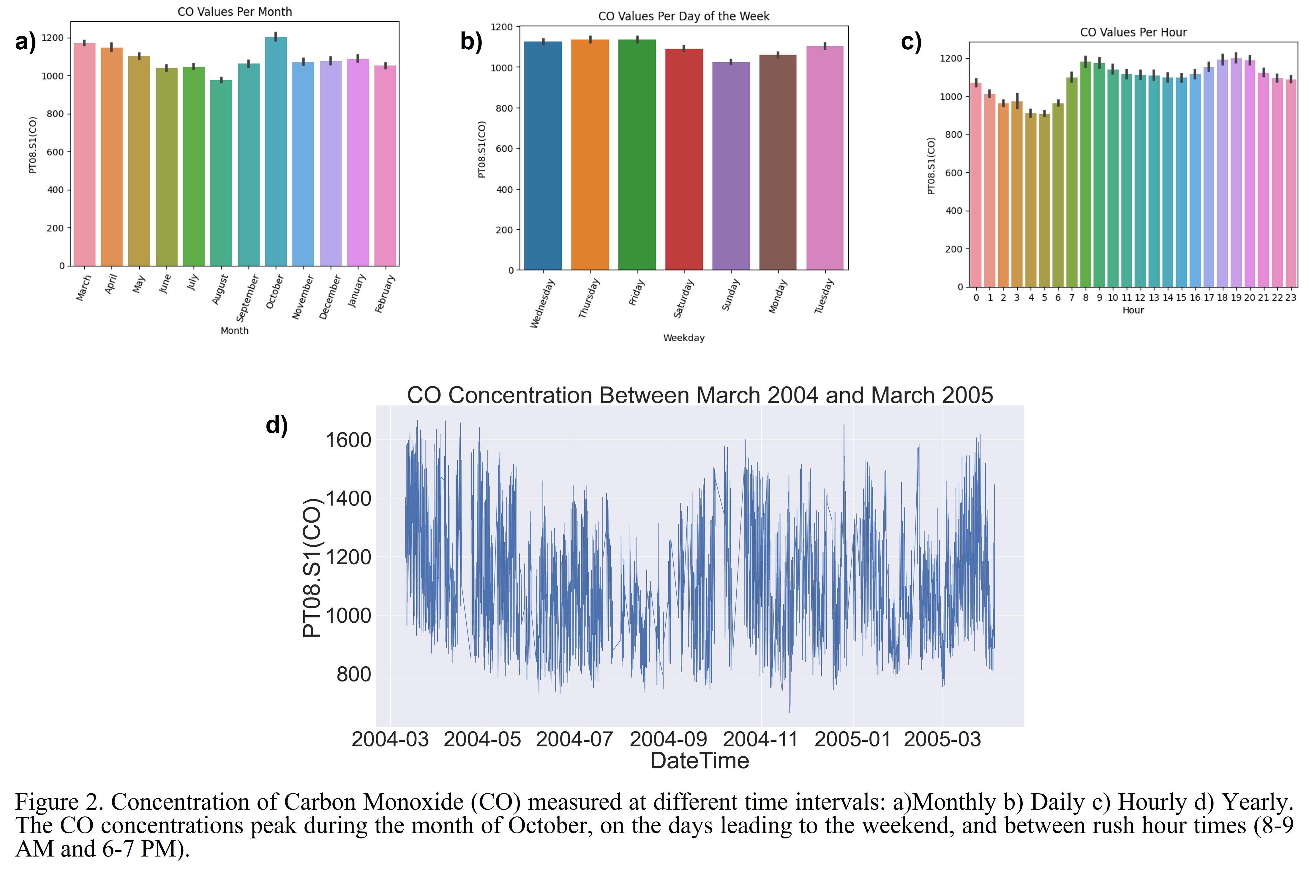
For instance, we can see that:
- October has the highest CO readings while August had the lowest readings.
- CO levels trend downward from October to August. They start to rise between August to October.
- CO levels are lowest on Sundays and highest on Friday.
- CO levels are lowest between 4-5 AM and highest at 8 AM and 7 PM.
Building and Assessing the Performance of Regressor Models
A total of 10 different regressors were used to build models to predict the concentrations of each pollutant. The data was split using the 80/20 Pareto principle for each regression model. The 10 regressors that were tested and the basic reasoning for trying them are:
- Linear Regression - Simple
- Huber Regression - Linear regression but robust to outliers
- Random Forest - High accuracy, scalable, and interpretable
- Gradient Boosting - Minimize bias error
- Gaussian Process - Non-parametric distribution
- K-Neighbors - Feature similarity
- Ada Boost - Powerful ensemble from simple model
- SVR - Account for non-linearity and highly tunable
- Decision Tree - Capture non-linearity
- MLP - Flexible
Model Results for CO Concentration
The results of the models built for the prediction of CO are shown below.
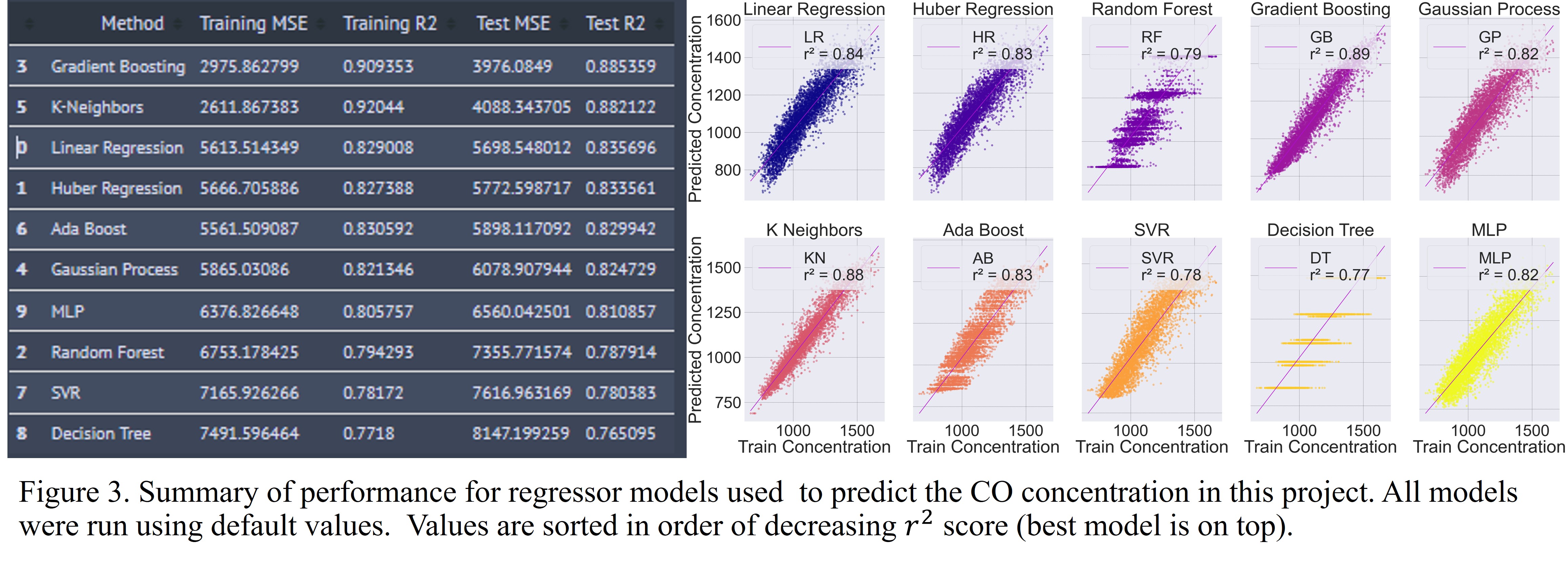
The Gradient Boosting regressor performed the best but it was closely followed by the K-Neighbors regressor. The Decision Tree showed the worst performance with the default values.
Model Results for NMHC Concentration
The results of the models built for the prediction of NMHC are shown below.
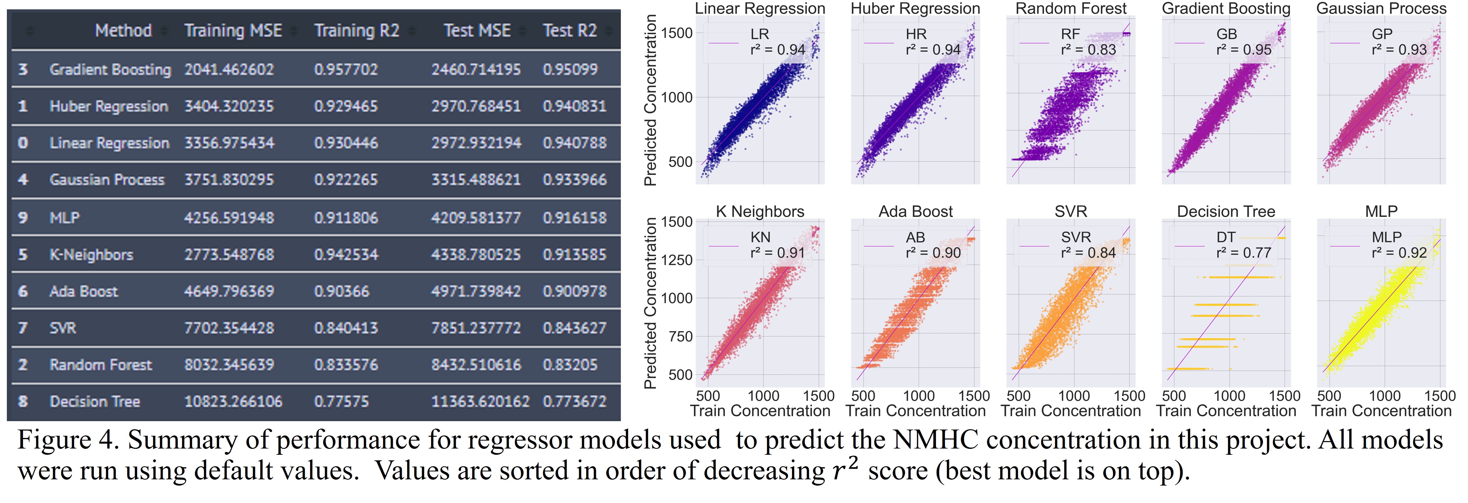
The Gradient Boosting regressor performed the best once again with an r2 score of 0.95 which is quite good. Huber Regression and Linear Regression were the next best performers. Decision Tree performed the worst once again.
Model Results for NO Concentration
The results of the models built for the prediction of NO are shown below.
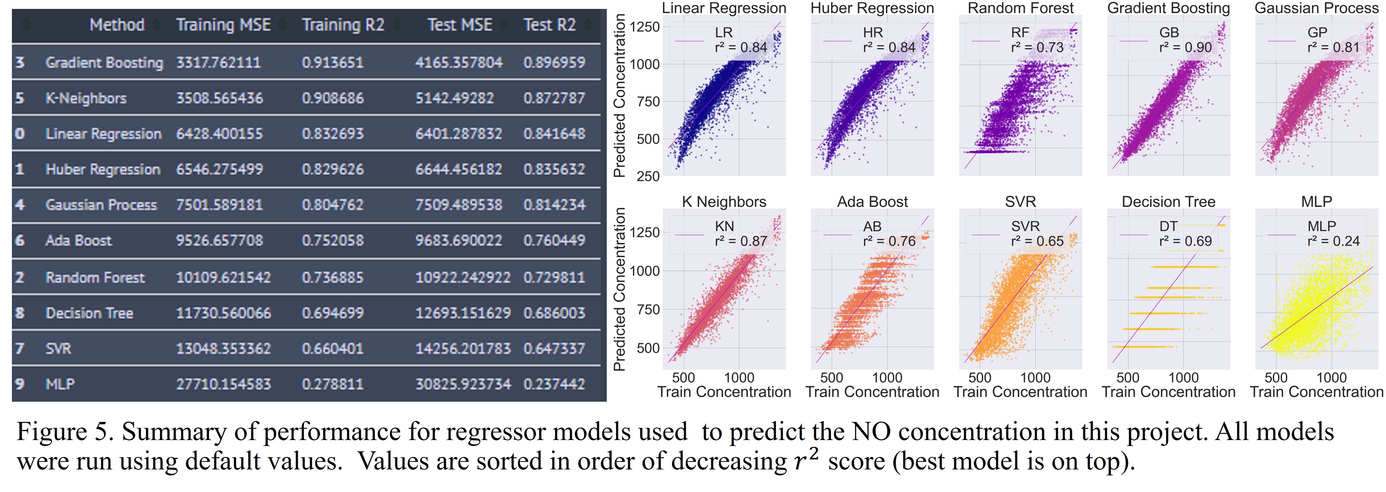
Yet again, the Gradient Boosting regressor performed the best with an r2 score of 0.90. It was closely followed by the K-Neighbors regressor. MLP performed extremely poorly with an r2 score of 0.24.
Model Results for NO2 Concentration
The results of the models built for the prediction of NO2 are shown below.

The Gradient Boosting regressor performed the best (again) with an r2 score of 0.95. Linear Regression and Huber Regression had the next best performance. SVR performed the worst with an r2 of 0.36.
Model Results for O3 Concentration
The results of the models built for the prediction of O3 are shown below.
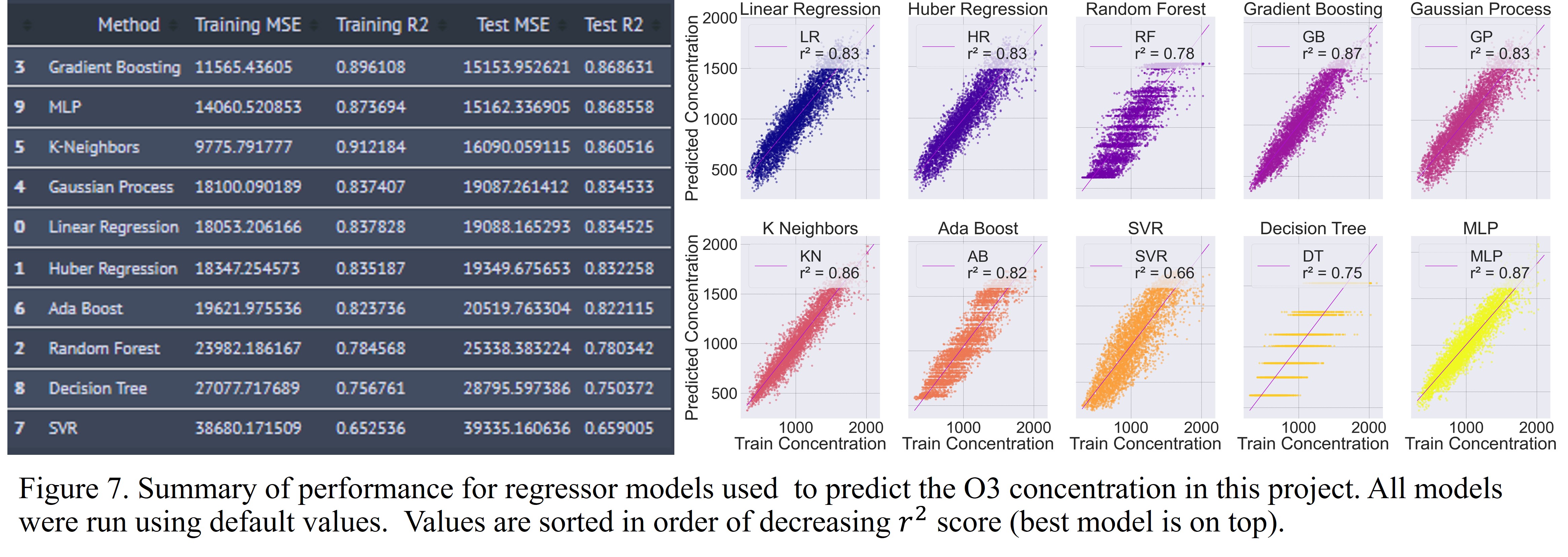
The Gradient Boosting regressor performed the best as has been the case with all the pollutants. MLP and K-Neighbors were the next best models. SVR performed the worst.
Summary of Models for Each Pollutant
The Gradient Boosting regressor model provided the best results based on the r2 score for all pollutants. Hence, I'll select it for further optimization through a grid-search parameter exploration.
Optimizing the Gradient Boosting Regressor Via Parameter Grid Search
Gradient Boosting (GB) is an ensemble model.
There's a few hyperparameters that can be tuned for the GB regressor. The results that I showed in the previous section were obtained by using the default parameters of the GB. There's 21 parameters that this regressor can take. You can see all those parameters here in the documentation.
The parameters I decided to try to optimize are as follows:
- learning_rate
- n_estimators
- max_depth
I decided to use the Mean Absolute Error (L1 Loss/MAE) as my loss function instead of the default value of Mean Squared Error since MAE is more robust to outliers.
I used a k-value of 5 for k-fold cross-validation. I also ran 8 calculations in parallel (1 for each CPU core in my computer) to expedite things.
You can see the results of the grid search exploration in the 3D scatter plot below. The grid search exploration took an hour and resulted in an improved r2 value of 0.91. A small increase, but an increase nonetheless.
The axes here correspond to the explored values for learning rate, n_estimators, and max_depth. The color scale represents the r2 score value. The brighter it is the better the model. The size of the markers represents the standard deviation of the model. Smaller values mean lower variance and viceversa. Therefore, the parameter combination I'm looking for will correspond to the smallest and brightest sphere.
A brief explanation of the effect of these parameters are shown below.
learning_rate determines the step size per each iteration that is made towards minimizing the value of the loss function. High learning rates can
overshoot the minima while low learning rates can lead to unfeasibly long convergence times and finding local minimum instead of the global minimum.
n_estimators refers to the number of trees used to build the model. In general, the higher this value the better the performance. However, as this value increases,
so does the computational time required for it to converge.
max_depth refers to number of nodes in the tree. The deeper the tree, the more splits is has and can thus capture more features in the data. If the number is too high though,
then we start running into issues of overfitting.
The results of the grid search exploration determined that the best parameters are:
- learning_rate = 0.1
- max_depth = 10
- n_estimators = 200
Predicting CO Concentration with Gradient Boosting Model On Entire Dataset
The plot below shows the final model predictions after evaluating the model on the entire dataset.

The plot shows the measured concentrations of CO as solid lines and the predicted concentrations of CO as dots after evalation on the entire
dataset over the course of 1 year. The model follows the data excellently and with high accuracy. This is further evidenced by the plots on the side that show that the residuals are normally distributed, that there is no heteroskedasticity present (i.e., the standard deviation is constant), and that the assumption of normally distributed residuals is correct.In other words, the generated model has high accuracy (low variance) and since it was able to fit the entire data population available, it also has low bias. This is the ideal situation.
I didn't show them here but a similar situation can be seen for the other 4 pollutants present in this dataset.
Conclusions and Final Thoughts
10 different machine learning regressor models were tested to determine which one predicted the pollutant concentration with th highest accuracy.
The Gradient Boosting (GB) Classifier had the highest prediction accuracy for all 5 pollutants explored within this data set.
The GB classifier was then optimized and cross-validated using the k-fold method through variation of the learning_rate, max_depth, and n_estimators hyperparamters.
The model was finally evaluated using the entire dataset which resulted in an r2 score of 1.0 which is excellent.
I had fun working on this project! It had a nice mix of time series analysis, use of statistical tools, model testing and optimization, and even some cool chemistry to top it off!
Something that I'd like to do in the future is implement this aproach for global data on pollutants to really test the limits of the model predictability.
Thanks for reading this and checking out my work!