Skip to content

Victor Murcia

• About
• Engineering
• Research
• Publications
• Writing
• Archive

Aug 23, 2022 · Archived

MNIST Image Classification with Convolutional Neural Network

Algorithm for mimicking the brain to recognize images

From earlier work — part of my archive of foundational machine-learning & data-science projects.

Image Classification with MNIST Dataset Using Artificial Neural Networks

This is going to be a quick showcase of how to perform Image Classification using a variety of techniques like multi-layer perceptron(MLP), convolutional neural networks (CNNs) and VGG16. The MNIST image database contains handwritten digits comprised of a training set of 60,000 examples and a test set of 10,000 examples. It is a great starting point for learning how to use a variety of neural network architectures. Here's a link to the dataset http://yann.lecun.com/exdb/mnist/

General Procedure for Using ANNs

Here is the general set of steps required to build a CNN for image classification:

1. Find and download a dataset
2. Load/Import the dataset into working environment
3. Familiarize yourself with data (i.e. display some images, get image shapes, how many images, etc.)
4. Preprocess the data (i.e., normalizize pixels, redimension as needed, one hot encoding, etc.)
5. Build the model (i.e., decide what layers to add and how they are made)
6. Determine what optimizer and loss function to use
7. Run the model
8. Assess the model

Modules Used in this Project

The two major modules in this project are tensorflow and keras. You can find the documentation for both of them below:

• https://www.tensorflow.org/api_docs/python/tf
• https://keras.io/api/

import tensorflow as tf

#For data preprocessing
from keras.preprocessing.image import ImageDataGenerator
from keras.utils import to_categorical #For one hot encoding

#For model building
from keras.models import Sequential, InputLayer
from keras.layers import Dense, Conv2D, Dropout, Flatten, MaxPooling2D

#For general plotting
import matplotlib.pyplot as plt

import random #To extract random images from dataset for plotting

Retrieiving the MNIST dataset

I'll start by downloading the MNIST dataset. This can be readily done with tensorflow without having to download it to my computer. I can also split my data into train and test sets via the code below:

(x_train, y_train), (x_test, y_test) = tf.keras.datasets.mnist.load_data()

Cool. Let's visualize our data really quick! I'll write a little routine below that will select 10 random images from the MNIST dataset and plot them along with their corresponding labels.

fig, axs = plt.subplots(1,10,figsize =(20,20)) 
for i in range(10): #Let me plot 10 random images from the dataset
    img_sel = random.randint(0, len(image_index))
    axs[i].imshow(x_train[img_sel], cmap='Greys')
    axs[i].set_title('Label ' + str(y_train[img_sel]), fontsize = 20)
plt.show()

Let's start getting some basic info about our dataset.

# summarize dataset shape
print('These are the dimensions for the Train and Test sets as well as their labels:')
print('Train', x_train.shape, y_train.shape)
print('Test' , x_test.shape, y_test.shape)
# summarize pixel values
print('These are the Min, Max, Average, and Standard Deviation of the images in the dataset:')
print('Train', x_train.min(), x_train.max(), x_train.mean(), x_train.std())
print('Test' , x_test.min() , x_test.max() , x_test.mean() , x_test.std())

These are the dimensions for the Train and Test sets as well as their labels:
Train (60000, 28, 28) (60000,)
Test (10000, 28, 28) (10000,)
These are the Min, Max, Average, and Standard Deviation of the images in the dataset:
Train 0 255 33.318421449829934 78.56748998339798
Test 0 255 33.791224489795916 79.17246322228644

The .shape function confirms that we have a training set comprised of 60,000 images and a test set composed of 10,000 images. We can also see that every image has dimensions of 28 x 28 pixels.

From, the statistics we calculated on these images we can see that the minimum pixel value is 0 and the maximum pixel value is 255. This is indicative of these images being in the RGB color space where 0 corresponds to black and 255 corresponds to white which makes sense based on the images I displayed earlier.

We can also see that there is some variance in the pixel colors which means that that our images are not composed of purely black and white pixels (i.e. there is some blurriness or shading in the images).

Finally, and importantly, we can see that the image data is currently set as a 3D array (i.e., the dataset size, image width and image length). We need to change it to a 4D array (this is called reshaping) to work with Keras. We also need to scale our data prior to doing any kind of neural network modeling.

Scaling Pixels

There are 3 main ways to accomplish pixel scaling: normalization, centering, and standardization. In pixel normalization the pixel values are scaled so that they fall in the range of 0-1. In pixel centering, pixel values are set to have a zero mean. Finally, in pixel standardization pixel values are set to have a zero mean and unit variance.

Normalization can be readily done in our case in two ways:

• By manually dividing the RGB channels by 255
• Ny using the ImageDataGenerator that comes with Keras

Regardless of the method we need to start by reshaping the training and testing sets as follow:

(x_train, y_train), (x_test, y_test) = tf.keras.datasets.mnist.load_data()

# Reshaping the array to 4-dims so that it can work with the Keras API
x_train = x_train.reshape(x_train.shape[0], 28, 28, 1)
x_test  = x_test.reshape(x_test.shape[0], 28, 28, 1)
input_shape = (28, 28, 1)

# Making sure that the values are float so that we can get decimal points after division
x_train = x_train.astype('float32')
x_test  = x_test.astype('float32')

Now I can simply divide these sets by 255 to get the normalized pixel values.

# Normalizing the RGB codes by dividing it to the max RGB value.
x_train /= 255
x_test  /= 255
print('x_train shape:', x_train.shape)

# summarize dataset shape
print('These are the dimensions for the Train and Test sets as well as their labels:')
print('Train', x_train.shape, y_train.shape)
print('Test' , x_test.shape, y_test.shape)

# summarize pixel values
print('These are the Min, Max, Average, and Standard Deviation of the images in the dataset:')
print('Train', x_train.min(), x_train.max(), x_train.mean(), x_train.std())
print('Test' , x_test.min() , x_test.max() , x_test.mean() , x_test.std())

x_train shape: (60000, 28, 28, 1)
These are the dimensions for the Train and Test sets as well as their labels:
Train (60000, 28, 28, 1) (60000,)
Test (10000, 28, 28, 1) (10000,)
These are the Min, Max, Average, and Standard Deviation of the images in the dataset:
Train 0.0 1.0 0.13066062 0.30810776
Test 0.0 1.0 0.13251467 0.31048027

The array for our training sets is now 4D and the pixel values are now within the range of 0-1.

The Keras image generator however has many built in methods that we can use to prep our data as we needed. I'll start by doing just normalization with the ImageGenerator which requires the rescale parameter.

(x_train, y_train), (x_test, y_test) = tf.keras.datasets.mnist.load_data()

# Reshaping the array to 4-dims so that it can work with the Keras API
x_train = x_train.reshape(x_train.shape[0], 28, 28, 1)
x_test  = x_test.reshape(x_test.shape[0], 28, 28, 1)

# one hot encode target values
y_train = to_categorical(y_train)
y_test  = to_categorical(y_test)

# Making sure that the values are float so that we can get decimal points after division
x_train = x_train.astype('float32')
x_test  = x_test.astype('float32')

# create generator
datagen = ImageDataGenerator(rescale=1.0/255.0)

Now I can use the flow function to load the image dataset in memory and generate batches of augmented data. This process is also referred to as generation of iterators. I'll be using a batch size of 64 which means that our dataset will be divided into groups of 64 images that will then be scaled via the iterators.

I should mention that batch size is as a hyperparameter and is thus wise to subject it to a grid search exploration during model development. In general though, it is common practice to use the largest batch size that the GPU will handle.

# prepare an iterators to scale images
train_iterator = datagen.flow(x_train, y_train, batch_size = 64)
test_iterator  = datagen.flow(x_test , y_test , batch_size = 64)
print('Batches train=%d, test=%d' % (len(train_iterator), len(test_iterator)))

# confirm the scaling works
batchX, batchy = train_iterator.next()
print('Batch shape=%s, min=%.3f, max=%.3f' % (batchX.shape, batchX.min(), batchX.max()))

Batches train=938, test=157
Batch shape=(64, 28, 28, 1), min=0.000, max=1.000

Nice! The min and the max values are 0 and 1 which means normalization worked! You can certainly more scaling conditions to your dataset and you can find more info here: https://www.tensorflow.org/api_docs/python/tf/keras/preprocessing/image/ImageDataGenerator

Building the Model

In CNNs we start with some input image. Then we assign the importance to different aspects/objects in the image. Finally, we can use weightings on these features to differentiate them from one another.

Images are simply arrays of numbers (aka matrices). Matrices can be treated as flattened vectors (i.e., a 3 x 3 matrix can be represented as a 1 x 9 vector). However, any image that has any kind of variations in their pixel definitions due to differences in colors, hues, saturation, brightness and such will not be properly caught by standard techniques due to the averaging process that ends up smearing the image properties and ultimately produces inaccurate results. In the CNN approach, this issue is not present due to the application of filters or layers into the image which preserves the spatial and temporal properties present in the image. This ultimately results in better training of datasets. Shown below is a visual depiction of an RGB color matrix. RGB matrices are composed of channels (i.e. layers) of Red, Blue, and Green. Each pixel in an image has an associated value extracted from each channel. The shape of these matrices is defined by the width and height of the image which in this case is 8 x 8 which results in an image made up of 64 pixels (each pixel will be an input and is also called a neuron in this context). An image made up of 64 pixels wouldn't be too computationally expensive to process, however the images that one is generally interested in classifying have a lot more features and pixels to assess which can rapidly get costly, complicated, and unfeasible.

CNNs deals with this cost and performance issue by reducing the size of the image into a more processable form while simultaneously producing accurate predictions. This is done via convolution and pooling layers

Convolution Matrices

A convolution matrix, also known as a convolution layer or a kernel, is the first place we extract image features like edges, color, and gradient orientation. The convolution process is depicted below. We start with the original image (9 x 9) on the left. Then, we take a convolution matrix of (3 x 3) that will be moved across the original image. Finally, a filtered image (7 x 7) is produced as an output.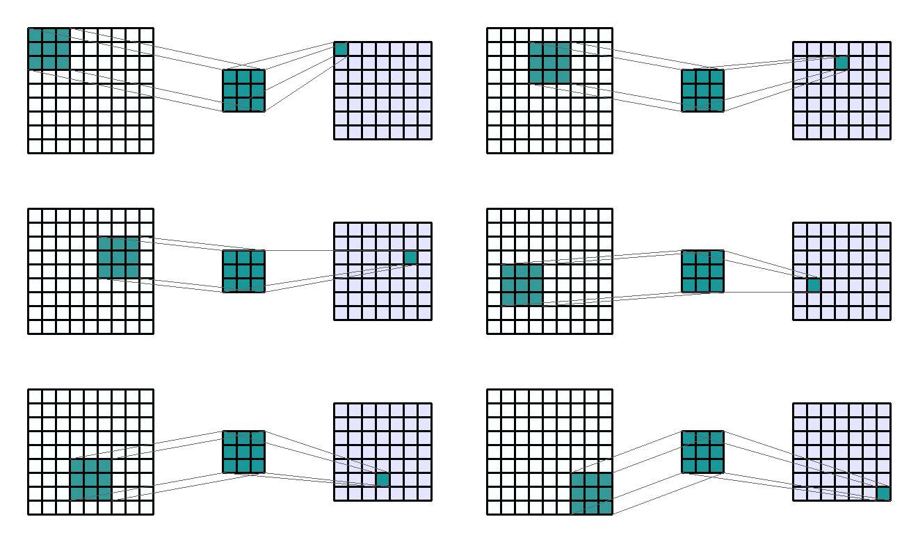

The size of the filtered image (assuming it is a square) due to convolution can be computed via the following formula

$Image Size = \frac{W-F+2P}{S} + 1$

Where W is the width of the original image, F is the size of the convolution matrix, P is the padding value, and S is the stride parameter. P and S are components of the model that I'll talk about later. For example, if an image is 75 × 75, a filter is 5 × 5, the padding is 3, and the stride is 2, the result of convolution will be:

$Image Size = \frac{75-5+2*3}{2} + 1 = 39$

In this example, we have reduced the image complexity from 5,625 pixels to 1,521 pixels which is a complexity reduction of 73%.

Pooling Matrices

In addition to the convolution matrix we'll also be applying a pooling matrix that will further reduce the size of the image we are processing which reduces the necessary computational power of the processing. The pooling matrix works in a similar way to the convolution matrix. The pooling process seeks to extract the dominant features from the convoluted image. There are two ways to construct the pooling matrix: Maximum Pooling and Average Pooling. In maximum pooling, the extracted value is the maximum value from the pooled region of the filtered image. In average pooling the extracted value is the average value from the pooled region of the filtered image. In general, max pooling performs better than average pooling since it discards noisy features while simultaneously reducing the dimensionality of the data. An example of the max pooling process is shown below where the orange matrix is the filtered image and the green matrix is the pooled matrix.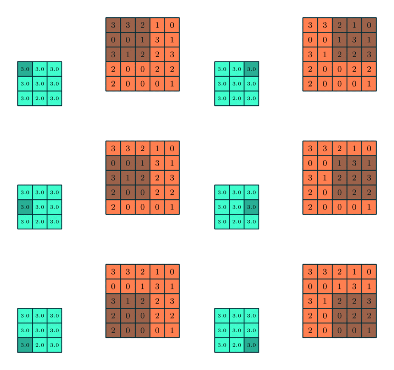

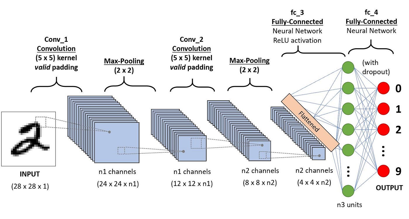
The convolutional layer and the pooling layer form a layer of a CNN. Multiple layers can be made from these. The model I'll be constructing here will consist of 2 layers.

Fully Connected Layers (FC Layer)

Now that we have a way to define our convolution and pooling layers. We can keep introduce the FC layer. The FC layer is essentially where the Network in Neural Networks comes into play. The FC layer allows the model parameters to be connected to our output in order to classify each image (i.e., give them a label). Mathematically, this is converting our multidimensional array into a column or row vector.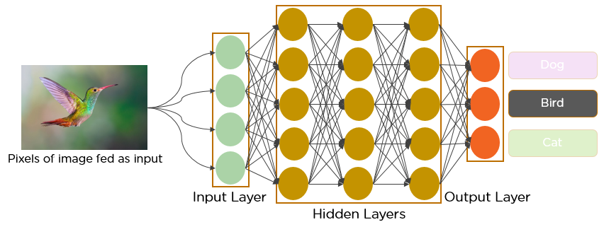

Dense Layers

Now that we have flattened our data through an FC layer we can start thinking about adding dense layers (DLs). A dense layer is a layer that is deeply connected to every neuron of the preceding layer and is created by matrix-vector multiplication as shown below:

$L = DF = \begin{bmatrix} a_{11} & a_{12} & ... & a_{1n}\\ a_{21} & a_{22} & ... & a_{2n} \\ \vdots & \vdots & \vdots & \vdots\\ a_{n1} & a_{n2} & ... & a_{nn} \end{bmatrix} \begin{bmatrix} b_{11}\\ b_{21}\\ \vdots\\ b_{n1} \end{bmatrix}$

The takeaway from this operation is that the application of dense layers results in further dimensionality reduction based on the neurons present in the previous layer.

Dropout Layers

The last layer I'll cover here is the dropout layer. The purpose of this layer is to minimize overfitting randomly setting the graph edges (i.e. neurons) on hidden layers to equal 0 during each update of the model training phase.

Phew! That's a fair bit to take in but now we are ready to start defining our neural network model.

Perceptron Neural Network

The first model architecture/structure I'll try is a perceptron (single neuron model). Perceptrons serve as the building block for larger and more complex neural networks. The perceptron we are initially building is made up of a single hidden layer.

• A dense layer from the original image
• Output --> layer composed of 10 neurons

(X_train, y_train), (X_test, y_test) = tf.keras.datasets.mnist.load_data()

number_pix = X_train.shape[1]**2

X_train = X_train.reshape(X_train.shape[0], number_pix).astype('float32')
X_test  = X_test.reshape(X_test.shape[0], number_pix).astype('float32')

X_train = X_train/255
X_test  = X_test/255

y_train = to_categorical(y_train)
y_test  = to_categorical(y_test)

num_classes=y_train.shape[1]

perc = Sequential()
perc.add(InputLayer(input_shape=(number_pix,)))
perc.add(Dense(number_pix, activation='relu'))
perc.add(Dense(num_classes, activation='softmax'))
perc.compile(loss='categorical_crossentropy', optimizer='adam', metrics=['accuracy'])
perc.summary()

Model: "sequential_64"
_________________________________________________________________
Layer (type)                 Output Shape              Param #   
=================================================================
dense_120 (Dense)            (None, 784)               615440    
_________________________________________________________________
dense_121 (Dense)            (None, 10)                7850      
=================================================================
Total params: 623,290
Trainable params: 623,290
Non-trainable params: 0
_________________________________________________________________

Even for a "simple" model like this we are still going to end up with over 600,000 parameters. Now let's run it!

perc.fit(X_train, y_train, validation_data=(X_test,y_test),epochs = 10, verbose=2)
score= perc.evaluate(X_test, y_test, verbose=0)
print('The error is: %.2f%%'%(100-score[1]*100))

Train on 60000 samples, validate on 10000 samples
Epoch 1/10
 - 16s - loss: 0.1896 - accuracy: 0.9442 - val_loss: 0.0964 - val_accuracy: 0.9703
Epoch 2/10
 - 16s - loss: 0.0756 - accuracy: 0.9764 - val_loss: 0.0789 - val_accuracy: 0.9742
Epoch 3/10
 - 16s - loss: 0.0489 - accuracy: 0.9851 - val_loss: 0.0692 - val_accuracy: 0.9789
Epoch 4/10
 - 16s - loss: 0.0347 - accuracy: 0.9891 - val_loss: 0.0741 - val_accuracy: 0.9761
Epoch 5/10
 - 16s - loss: 0.0252 - accuracy: 0.9915 - val_loss: 0.0667 - val_accuracy: 0.9809
Epoch 6/10
 - 16s - loss: 0.0211 - accuracy: 0.9933 - val_loss: 0.0716 - val_accuracy: 0.9805
Epoch 7/10
 - 16s - loss: 0.0181 - accuracy: 0.9937 - val_loss: 0.1000 - val_accuracy: 0.9749
Epoch 8/10
 - 16s - loss: 0.0127 - accuracy: 0.9957 - val_loss: 0.0680 - val_accuracy: 0.9834
Epoch 9/10
 - 16s - loss: 0.0140 - accuracy: 0.9950 - val_loss: 0.1078 - val_accuracy: 0.9776
Epoch 10/10
 - 16s - loss: 0.0108 - accuracy: 0.9964 - val_loss: 0.0836 - val_accuracy: 0.9810
The error is: 1.90%

Nice! This simple model has an accuracy of 98.1% already! Let's try a CNN now.

Convolutional Neural Network

• I'll start by using the Sequential() class. A Sequential model is appropriate for a plain stack of layers where each layer has exactly one input tensor and one output tensor. Here we are inputting an image composed of pixels and outputting a label.
• 2 layers composed of a convolutional layer and a pooling layer each
• 1 FC layer
• A dense layer
• 1 dropout layer
• Final dense layer composed of 10 neurons

(x_train, y_train), (x_test, y_test) = tf.keras.datasets.mnist.load_data()

#Preprocessing data for CNN
# Reshaping the array to 4-dims so that it can work with the Keras API
x_train = x_train.reshape(x_train.shape[0], 28, 28, 1)
x_test  = x_test.reshape(x_test.shape[0], 28, 28, 1)

# one hot encode target values
y_train = to_categorical(y_train)
y_test  = to_categorical(y_test)

# Making sure that the values are float so that we can get decimal points after division
x_train = x_train.astype('float32')
x_test  = x_test.astype('float32')

# create generator
datagen = ImageDataGenerator(rescale=1.0/255.0)

# prepare an iterators to scale images
train_iterator = datagen.flow(x_train, y_train, batch_size = 64)
test_iterator  = datagen.flow(x_test , y_test , batch_size = 64)
print('Batches train=%d, test=%d' % (len(train_iterator), len(test_iterator)))

# confirm the scaling works
batchX, batchy = train_iterator.next()
print('Batch shape=%s, min=%.3f, max=%.3f' % (batchX.shape, batchX.min(), batchX.max()))

# define model
input_shape = (28, 28, 1) #Each image is 28 x 28 pixels and composed of single layer
model = Sequential()

#First layer has a 3x3 convolution matrix and a 2x2 pooling matrix. Number of channels is 64.
model.add(Conv2D(64, (3, 3), activation='relu', input_shape = input_shape))
model.add(MaxPooling2D((2, 2)))

#Second layer has a 3x3 convolution matrix  and a 2x2 pooling matrix. Number of channels is 64.
model.add(Conv2D(64, (3, 3), activation='relu'))
model.add(MaxPooling2D((2, 2)))

#Generate FC Layer for Classification
model.add(Flatten())

#Add a dense layer
model.add(Dense(64, activation='relu'))

#Add a dropout layer to prevent/minimize overfitting
model.add(Dropout(0.2))

#Add the final dense layer composed of 10 neurons
model.add(Dense(10, activation='softmax')) #10 neurons in the end because numbers are from 0-9

Batches train=938, test=157
Batch shape=(64, 28, 28, 1), min=0.000, max=1.000

Sweet! We now have an unoptimized CNN that's almost ready to be fitted to our training dataset. Here's the model summary.

model.summary()

Model: "sequential_5"
_________________________________________________________________
Layer (type)                 Output Shape              Param #   
=================================================================
conv2d_9 (Conv2D)            (None, 26, 26, 64)        640       
_________________________________________________________________
max_pooling2d_9 (MaxPooling2 (None, 13, 13, 64)        0         
_________________________________________________________________
conv2d_10 (Conv2D)           (None, 11, 11, 64)        36928     
_________________________________________________________________
max_pooling2d_10 (MaxPooling (None, 5, 5, 64)          0         
_________________________________________________________________
flatten_5 (Flatten)          (None, 1600)              0         
_________________________________________________________________
dense_8 (Dense)              (None, 64)                102464    
_________________________________________________________________
dropout_2 (Dropout)          (None, 64)                0         
_________________________________________________________________
dense_9 (Dense)              (None, 10)                650       
=================================================================
Total params: 140,682
Trainable params: 140,682
Non-trainable params: 0
_________________________________________________________________

Compiling the model

I'll compile the model now where I'll add prameters like an optimizer, the loss functtion, and the accuracy metric.

# compile model
model.compile(optimizer='adam', loss='categorical_crossentropy', metrics=['accuracy'])

Fitting and Evaluating the Model

Now that we have preprocessed our data and defined a model we can now go ahead and try to fit it. This is done via the fit_generator function in keras where we can define things like how many epochs and steps_per_epoch to use. Let's run it and see what happens!

# fit model with generator
model.fit_generator(train_iterator, steps_per_epoch=len(train_iterator), epochs=5)

Epoch 1/5
938/938 [==============================] - 22s 23ms/step - loss: 0.2059 - accuracy: 0.9379
Epoch 2/5
938/938 [==============================] - 21s 23ms/step - loss: 0.0671 - accuracy: 0.9803
Epoch 3/5
938/938 [==============================] - 21s 22ms/step - loss: 0.0482 - accuracy: 0.9857
Epoch 4/5
938/938 [==============================] - 21s 23ms/step - loss: 0.0366 - accuracy: 0.98800s - loss: 0.0368 - accuracy
Epoch 5/5
938/938 [==============================] - 21s 22ms/step - loss: 0.0310 - accuracy: 0.9904

<keras.callbacks.callbacks.History at 0x249aeb2ec08>

# evaluate model
_, acc = model.evaluate_generator(test_iterator, steps=len(test_iterator), verbose=0)
print('Test Accuracy: %.3f' % (acc * 100))

Test Accuracy: 99.100

Look at that! The model accuracy is 99.1%. Pretty neat!

VGG16 Implementation

VGG16 is a convolution neural net (CNN) architecture that is considered to be one of the best computer vision models available. The architecture of VGG16 is composed of 16 different layers which generates approximately 134 million parameters. This model is absolutely overkill for this dataset but I'll build it here just for practice. The structure of VGG16 is as follows: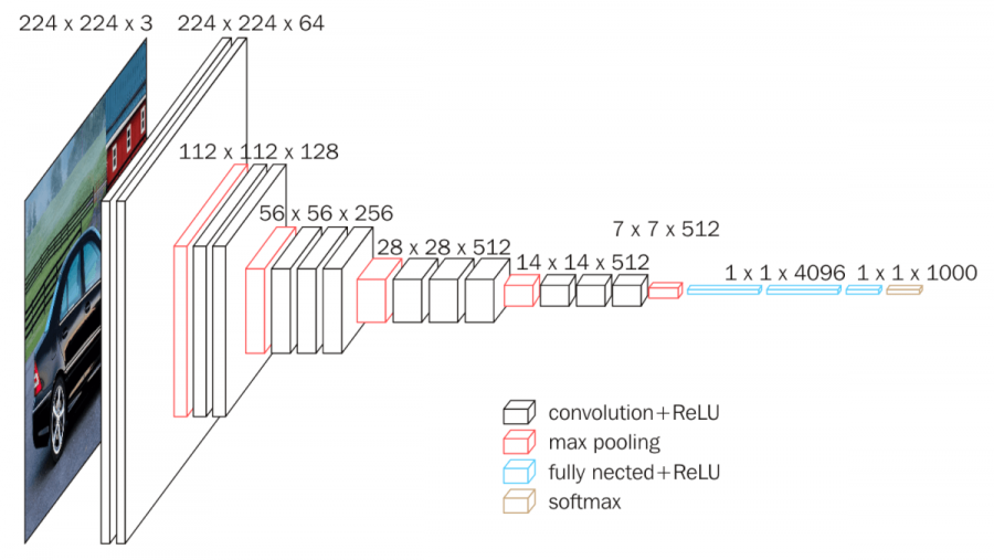

• 2x Convolution Layers + 1x Max Pooling
• 2x Convolution Layers + 1x Max Pooling
• 3x Convolution Layers + 1x Max Pooling
• 3x Convolution Layers + 1x Max Pooling
• 3x Convolution Layers + 1x Max Pooling
• 3 FC Layers
• Output --> 1 Dense Layer with SoftMax

We can build it our model as shown below. I had to use the padding = 'same' specifcation for the MaxPool2D layers since our images are fairly small which results in negative dimensions because calculated at the end...

from keras.layers import  MaxPool2D
(x_train, y_train), (x_test, y_test) = tf.keras.datasets.mnist.load_data()

#Preprocessing data for CNN
# Reshaping the array to 4-dims so that it can work with the Keras API
x_train = x_train.reshape(x_train.shape[0], 28, 28, 1)
x_test  = x_test.reshape(x_test.shape[0], 28, 28, 1)

# one hot encode target values
y_train = to_categorical(y_train)
y_test  = to_categorical(y_test)

# Making sure that the values are float so that we can get decimal points after division
x_train = x_train.astype('float32')
x_test  = x_test.astype('float32')

# create generator
datagen = ImageDataGenerator(rescale=1.0/255.0)

# prepare an iterators to scale images
train_iterator = datagen.flow(x_train, y_train, batch_size = 64)
test_iterator  = datagen.flow(x_test , y_test , batch_size = 64)
print('Batches train=%d, test=%d' % (len(train_iterator), len(test_iterator)))

# confirm the scaling works
batchX, batchy = train_iterator.next()
print('Batch shape=%s, min=%.3f, max=%.3f' % (batchX.shape, batchX.min(), batchX.max()))

# define model
input_shape = (28, 28, 1) #Each image is 28 x 28 pixels and composed of single layer
model = Sequential()

#Layer 1-2 64 channel 
model.add(Conv2D(input_shape=input_shape,filters=64,kernel_size=(3,3),padding="same", activation="relu"))
model.add(Conv2D(filters=64,kernel_size=(3,3),padding="same", activation="relu"))
model.add(MaxPool2D(pool_size=(2,2),strides=(2,2)))

#Layer 3-4 128 channel
model.add(Conv2D(filters=128, kernel_size=(3,3), padding="same", activation="relu"))
model.add(Conv2D(filters=128, kernel_size=(3,3), padding="same", activation="relu"))
model.add(MaxPool2D(pool_size=(2,2),strides=(2,2)))

#Layer 5-7 256 channel
model.add(Conv2D(filters=256, kernel_size=(3,3), padding="same", activation="relu"))
model.add(Conv2D(filters=256, kernel_size=(3,3), padding="same", activation="relu"))
model.add(Conv2D(filters=256, kernel_size=(3,3), padding="same", activation="relu"))
model.add(MaxPool2D(pool_size=(2,2),strides=(2,2)))
#Layer 8-10 512 channel
model.add(Conv2D(filters=512, kernel_size=(3,3), padding="same", activation="relu"))
model.add(Conv2D(filters=512, kernel_size=(3,3), padding="same", activation="relu"))
model.add(Conv2D(filters=512, kernel_size=(3,3), padding="same", activation="relu"))
model.add(MaxPool2D(pool_size=(2,2),strides=(2,2)))

#Layer 11-13 512 channel
model.add(Conv2D(filters=512, kernel_size=(3,3), padding="same", activation="relu"))
model.add(Conv2D(filters=512, kernel_size=(3,3), padding="same", activation="relu"))
model.add(Conv2D(filters=512, kernel_size=(3,3), padding="same", activation="relu"))
model.add(MaxPool2D(pool_size=(2,2),strides=(2,2), padding='same'))

#Layer 14 FC Layer
model.add(Flatten())

#Layer 15 Dense Layer
model.add(Dense(units=4096,activation="relu"))

#Layer 16 Dense Layer
model.add(Dense(units=4096,activation="relu"))

#Output Layer --> Final Dense Layer with softmaz
model.add(Dense(units=10, activation="softmax"))

Batches train=938, test=157
Batch shape=(64, 28, 28, 1), min=0.000, max=1.000

from keras.optimizers import Adam
opt = Adam(lr = 0.001)
model.compile(optimizer=opt, loss = 'categorical_crossentropy', metrics=['accuracy'])
model.summary()

Model: "sequential_66"
_________________________________________________________________
Layer (type)                 Output Shape              Param #   
=================================================================
conv2d_184 (Conv2D)          (None, 28, 28, 64)        640       
_________________________________________________________________
conv2d_185 (Conv2D)          (None, 28, 28, 64)        36928     
_________________________________________________________________
max_pooling2d_78 (MaxPooling (None, 14, 14, 64)        0         
_________________________________________________________________
conv2d_186 (Conv2D)          (None, 14, 14, 128)       73856     
_________________________________________________________________
conv2d_187 (Conv2D)          (None, 14, 14, 128)       147584    
_________________________________________________________________
max_pooling2d_79 (MaxPooling (None, 7, 7, 128)         0         
_________________________________________________________________
conv2d_188 (Conv2D)          (None, 7, 7, 256)         295168    
_________________________________________________________________
conv2d_189 (Conv2D)          (None, 7, 7, 256)         590080    
_________________________________________________________________
conv2d_190 (Conv2D)          (None, 7, 7, 256)         590080    
_________________________________________________________________
max_pooling2d_80 (MaxPooling (None, 3, 3, 256)         0         
_________________________________________________________________
conv2d_191 (Conv2D)          (None, 3, 3, 512)         1180160   
_________________________________________________________________
conv2d_192 (Conv2D)          (None, 3, 3, 512)         2359808   
_________________________________________________________________
conv2d_193 (Conv2D)          (None, 3, 3, 512)         2359808   
_________________________________________________________________
max_pooling2d_81 (MaxPooling (None, 1, 1, 512)         0         
_________________________________________________________________
conv2d_194 (Conv2D)          (None, 1, 1, 512)         2359808   
_________________________________________________________________
conv2d_195 (Conv2D)          (None, 1, 1, 512)         2359808   
_________________________________________________________________
conv2d_196 (Conv2D)          (None, 1, 1, 512)         2359808   
_________________________________________________________________
max_pooling2d_82 (MaxPooling (None, 1, 1, 512)         0         
_________________________________________________________________
flatten_18 (Flatten)         (None, 512)               0         
_________________________________________________________________
dense_124 (Dense)            (None, 4096)              2101248   
_________________________________________________________________
dense_125 (Dense)            (None, 4096)              16781312  
_________________________________________________________________
dense_126 (Dense)            (None, 10)                40970     
=================================================================
Total params: 33,637,066
Trainable params: 33,637,066
Non-trainable params: 0
_________________________________________________________________

model.fit_generator(train_iterator, steps_per_epoch = len(train_iterator), epochs=5)

Epoch 1/5
938/938 [==============================] - 1689s 2s/step - loss: 2.3016 - accuracy: 0.1108
Epoch 2/5
938/938 [==============================] - 1697s 2s/step - loss: 2.3014 - accuracy: 0.1124
Epoch 3/5
938/938 [==============================] - 1677s 2s/step - loss: 2.3014 - accuracy: 0.1124
Epoch 4/5
938/938 [==============================] - 1655s 2s/step - loss: 2.3013 - accuracy: 0.1124
Epoch 5/5
938/938 [==============================] - 1652s 2s/step - loss: 2.3013 - accuracy: 0.1124

<keras.callbacks.callbacks.History at 0x24af68ddc88>

Yikes... that didn't work too well... It also took much longer than the Perceptron or regular CNN. I wonder why it performed so poorly? I'll have to look deeper into this...

Conclusions

Three different ANN models (MLP, CNN, VGG16) were trained using the MNIST dataset. The best performing model resulted in a 99.1% accuracy classification. The elements shown here can be readily applied to other datasets and I'm interested in seeing what other things I can classify. I'll also be working towards applying other ANN methods like Deep Learning and Deep Dream as well as working on other datasets. :]

References

• https://towardsdatascience.com/conv2d-to-finally-understand-what-happens-in-the-forward-pass-1bbaafb0b148
• https://jamesmccaffrey.wordpress.com/2018/05/30/convolution-image-size-filter-size-padding-and-stride/
• https://www.guru99.com/tensor-tensorflow.html
• https://towardsdatascience.com/machine-learning-part-20-dropout-keras-layers-explained-8c9f6dc4c9ab
• https://analyticsindiamag.com/a-complete-understanding-of-dense-layers-in-neural-networks/
• https://machinelearningmastery.com/how-to-normalize-center-and-standardize-images-with-the-imagedatagenerator-in-keras/
• https://towardsdatascience.com/image-classification-in-10-minutes-with-mnist-dataset-54c35b77a38d
• https://towardsdatascience.com/a-comprehensive-guide-to-convolutional-neural-networks-the-eli5-way-3bd2b1164a53
• https://studymachinelearning.com/keras-imagedatagenerator-with-flow/
• https://itk.org/ITKSoftwareGuide/html/Book1/ITKSoftwareGuide-Book1ch6.html
• https://keras.io/guides/sequential_model/
• https://towardsdatascience.com/convolutional-neural-network-feature-map-and-filter-visualization-f75012a5a49c
• https://www.analyticsvidhya.com/blog/2021/05/convolutional-neural-networks-cnn/

---

← Back to the archive

Victor Murcia, PhD AI Engineering · Scientific Computing · Technical Leadership

GitHub LinkedIn arXiv RSS

© 2026 Victor Murcia