Spam is annoying and over time, it also serves as incremental waste of time. Even if it only takes a few seconds to delete a spam email, if left unchecked, spam will rapidly flood your inbox which can make the time spend handling spam add up fast.
In addition to the time-wasting component, spam can be dangerous since they are often embedded with fraudulent links and riddled with viruses than can do some serious damage to our computers, finances, and identity. As such, having a reliable way to deal with it is extremely important.
In this project, I'll be using the spambase dataset in conjunction with machine learning techniques to develop a model that accurately classifies email as spam or not spam.
If you'd like to see all of my work in this project you can find it in the repository found here.
Exploratory Data Analysis
The spambase includes 57 features (columns) and 4601 e-mails (rows). Its features are characterized as follows:- word_freq_WORD - percentage of words in the e-mail that match WORD.
- char_freq_CHAR - percentage of characters in the e-mail that match the symbol CHAR.
- capital_run_length_average - average lenth of uninterrupted sequences of capital letters.
- capital_run_length_longest - length of longest uninterrupted sequence of catipal letters.
- capital_run_length_total - total number of capital letters in the email.
- class - denotes whether the e-mail was considered spam (1) or not (0)
The features are all numerical (54 are continuous real and 3 are continuous integer). The target variable is categorical and nominal. Given this, ANOVA is likely the best suited feature selection method to carry out dimensionality reduction.
This is a binary classification problem so I want to ensure that the class distribution is evenly split before continuing in order to determine how to proceed further. The plot below shows the counts, frequency, and percent of the spam class.
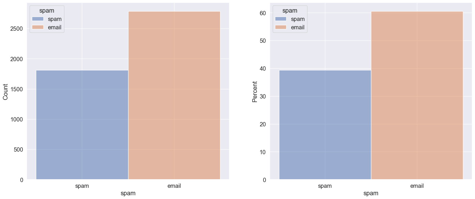
As can be seen above, 60% of the emails in the dataset are classified as non-spam while 40% are classified as spam. This is not an extremely inbalanced dataset but it means that cross-validation will be necessary for accurate sampling.
Dimensionality Reduction Through ANOVA
The process of simplifying a model through dimensionality reduction can help in facilitating the explainability of the model and minimizing over-fitting. The spambase dataset contains 57 features, however, I'd like to start with a much smaller number of features and see how accurate of a model I can generate. To accomplish this initial reduction in dimensionality I will use the ANOVA test since my features are continuous numerical and my dependent variable is nominal.
F-Scores are a measure of how informative a feature is for a dataset as calculated from the ANOVA test. The higher the F-Score the more informative the feature is. The results for this first ANOVA test are shown below.
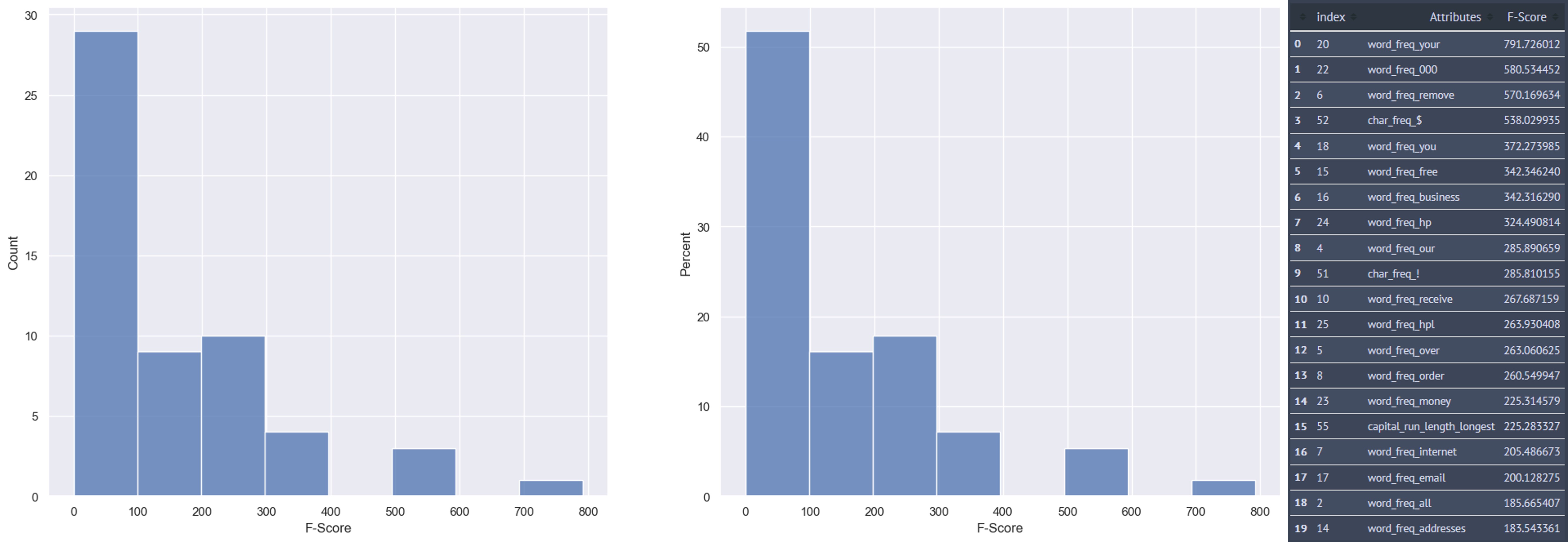
As can be seen from the plots above, over 50% of the features have F-scores between 0-100 which are low. The features with the highest F-scores are located in the last 3 bins which have values ranging between 300-800. The number of features that match this criteria are 8. Therefore, I'll use those 8 features as my initial set of features for the model and see how it performs.
Below we can see the pandas_profiling report for initial reduced dataset.
Testing Different Classification Models
I'll test out 11 different classification models to see which one performs best. The data will be split using an 80/20 split and the models will be run using their default parameters to start off.
The models I'll be testing are shown below
- Linear Perceptron
- Gaussian Naive Bayes
- Random Forest
- Bagging Classifier
- Extreme Gradient
- K-Neighbors
- Decision Tree
- Extreme Gradient Boosting
- Gaussian Process
- Support Vector
- MLP
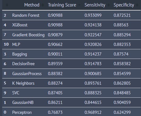
The results are shown in the tables below
The first table has the results from each of the models sorted in order of descending accuracy score. The Random Forest, XGBoost, and Gradient Boosting Classifiers were the top 3 performers.
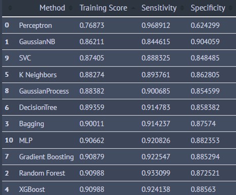
The second table has the results from each of the models sorted in order of descending sensitivity score. The Perceptron, Gaussian Naive Bayes, and SVC Classifiers were the top 3 performers.
The third table has the results from each of the models sorted in order of descending specificity score. The Gaussian Naive Bayes, XGBoost and Gradient Boosting Classifiers were the top 3 performers.
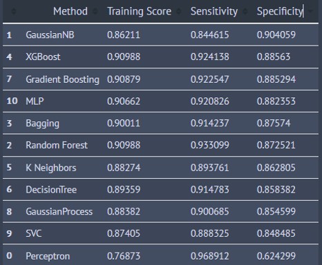
Which model should I choose is going to be based on whether I want to maximize sensitivity or specificity. The equations specificity and sensitivity are shown below
Specificity is known as the True Negative Rate. When the value of specificity is high then the model is good at predicting true negatives.

Sensitivity is known as the True Positive Rate. When the value of sensitivity is high then the model is good at predicting true positives.

A false positive in this case entails a non-spam email being classified as spam.
A false negative in this case entails a spam email not being classified as spam.
From the scenarios above, it is clear that classifiying a non-spam email as spam is worse than classifying a spam email as non-spam. Therefore, I'll need to maximize specificity.
The models with the highest specificity are the Gaussian Naive Bayes (GNB) and the XGBoost (XGB) classifiers.
The confusion matrices for the GNB (left) and the XGB (right) classifiers are show below.
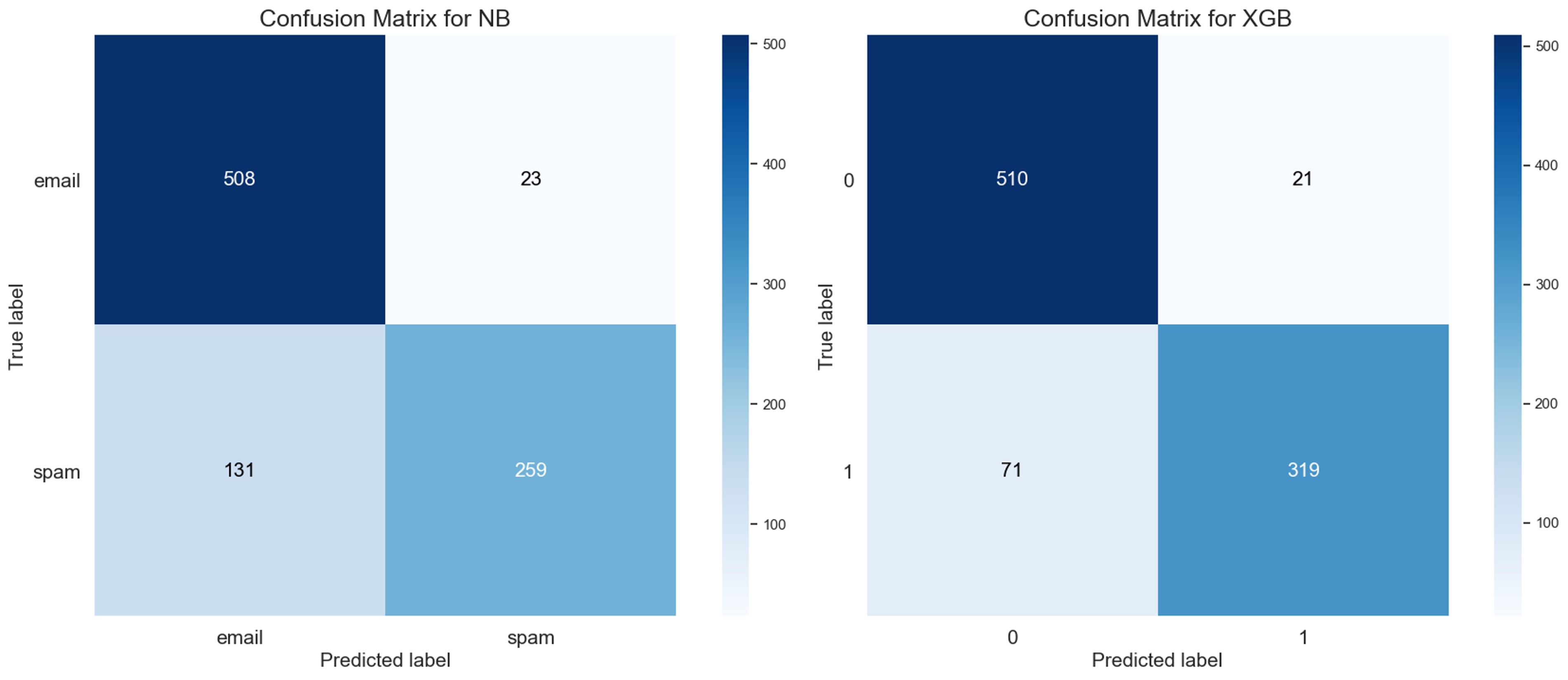
From these matrices we can see the following:
- The GNB resulted in 23 false positives and 131 false negatives
- The XGB resulted in 21 false positives and 71 false negatives
Hmm, the XGB classifier has a better distribution of false positives/negatives so I'll refine it further through cross-validation and a parameter grid-search.
Optimizing the XGB Classifier
The performance of the XGBoost classifier is already quite good. However, it could certainly be improved through a parameter space exploration. There's quite a few parameters at our disposal to tune for XGBoost which you can find in the documentation.
I decided to explore and optimize the following parameters and see if an even better performance can be achieved:
- learning_rate
- max_depth
- n_estimators
For this grid search I used a k-fold cross-validation set to k=10 and optimized via the accuracy, precision, and recall scores.
The parameter space exploration improved the accuracy and specificity scores of the XGB Classifier. The accuracy score increased to 0.98 which is a marked improvement from the 0.91 score I started off with. The sensitivity remained the same (0.92) while the specificity increased to 0.92 from 0.89. The confusion matrix is shown below.
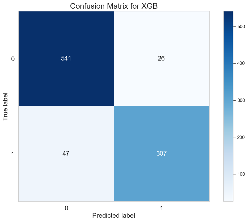
From this matrix we can see the following:
- The XGB resulted in 26 false positives and 47 false negatives. It also has 541 true positives and 307 true negatives.
Even though the number of false positives increased slightly, the accuracy and the precision of the model are much better now.
Let me look at the separability of the model by checking the ROC-AUC curve as shown below.
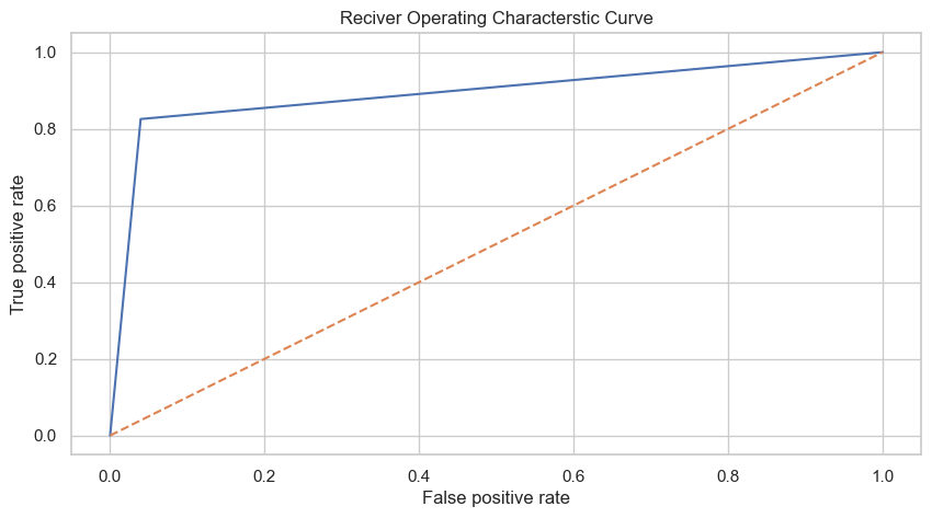
Hmm, the AUC of this model is 0.89 which isn't terrible but could and should be improved. If the separability of the model is improved then, the number of false positive/negative classifications should also go down since more separability is indicative of better distinction between the target classes.
I ran another grid-search where I sought to improve the AUC score and the accuracy score, but I didn't obtain the improvement I was looking for. The AUC improved to 0.91 but the accuracy dropped a bit. For this reason, I decided to increase the size of the model and see if I get better results this way.
I also tried to incorporate more features into the model and carried out the same analysis as shown above but did not obtain much improvement. I'll be using the larger model for the rest of the analysis.
Explaining the Model
Let's see how the model decided how to make a classification for spam. The table below shows the weights of each feature present in the model. As can be seen, The word_freq_hp,word_freq_remove and the capital_run_length_longset were the top 3 features contributing to the final classification of spam.From the partial dependence plots below we can see how each of these features contributed towards assessing whether an email is spam or not.
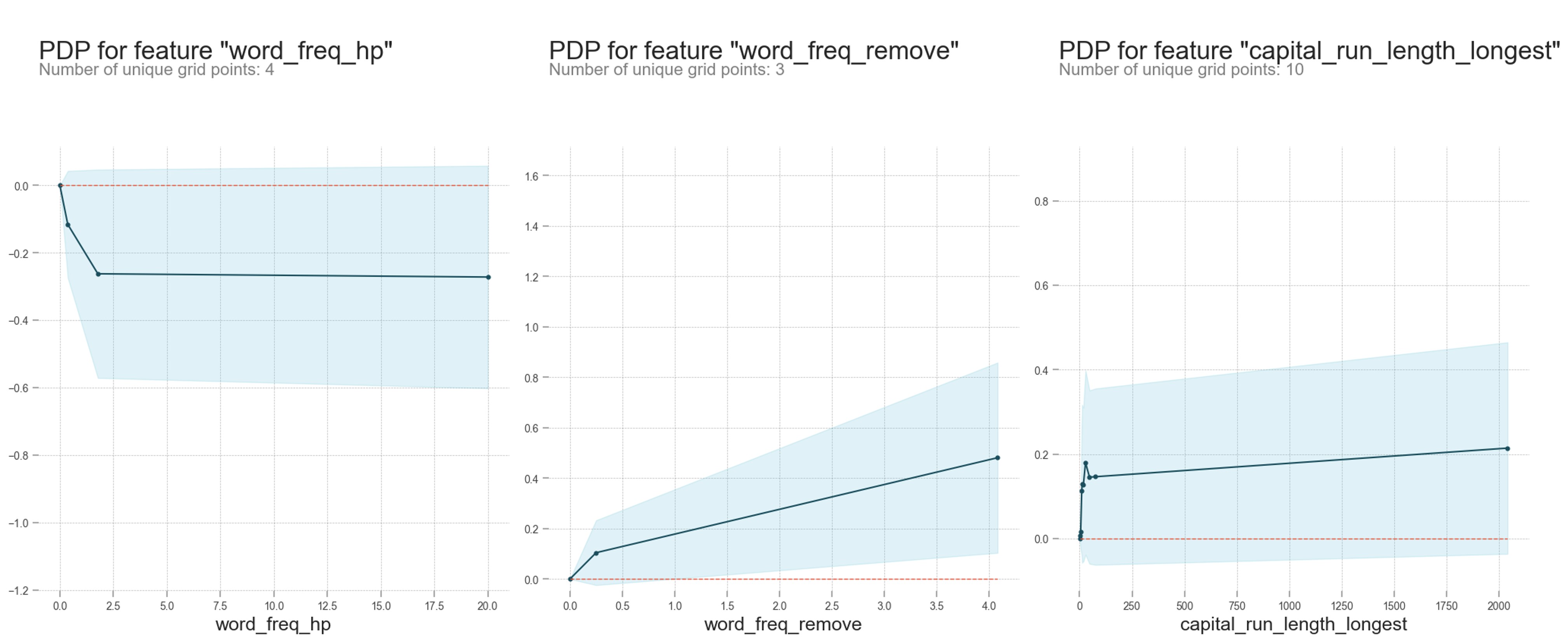
From the PDPs we can see the following:
- The probability of an email being spam decreases if the frequency of the word 'hp' in the email increases
- The probability of an email being spam increases if the frequency of the word 'remove' in the email increases
- The probability of an email being spam increases if the length of longest uninterrupted sequence of capital letters in the email increases
The data comes from a Hewlett-Packard Technical Report. Hence, the frequent presence of 'hp' in the email could be considered a good sign that the email is not spam since it could be indicative of an internal company email. A higher frequency of the word remove leading to a more likely spam email can also make sense since a spammer/hacker could be asking the users to remove things like an antivirus or a firewall which is generally a bad idea. Lastly, having more capital letters stringed together is usually a sign of spam emails since these emails often have little to no proofreading and are riddled with all sorts of orthographic mistakes.
These, decisions all make sense to me and if I were the one trying to decide whether an email is spam, those are certainly things that I would strongly consider towards classifying an email as spam.
Let's look at the 2D PDPs to see how these features interact to produce the classification. The 2D PDP plots below will show the interactions of the top 3 features in the mdoel. The color scale in the plots below represents the probability of an email being classified as spam. Blue colors mean lower probability of spam while red colors represent higher probability of spam.

From the 2D PDP plots we can see the following:
- The probability of an email being spam is highest when the word remove is in the email for all lengths of sequential capital letters
- The proability of an email being spam is highest when the word hp has a low frequency and the lengths of sequential capital letters is long
- The proability of an email being spam is highest when the word hp has a low frequency and the frequency of the word remove is high
Let me look at the SHAP values. SHAP values allow us to understand the impact from each feature in our model by breaking down the predictions made by the model.
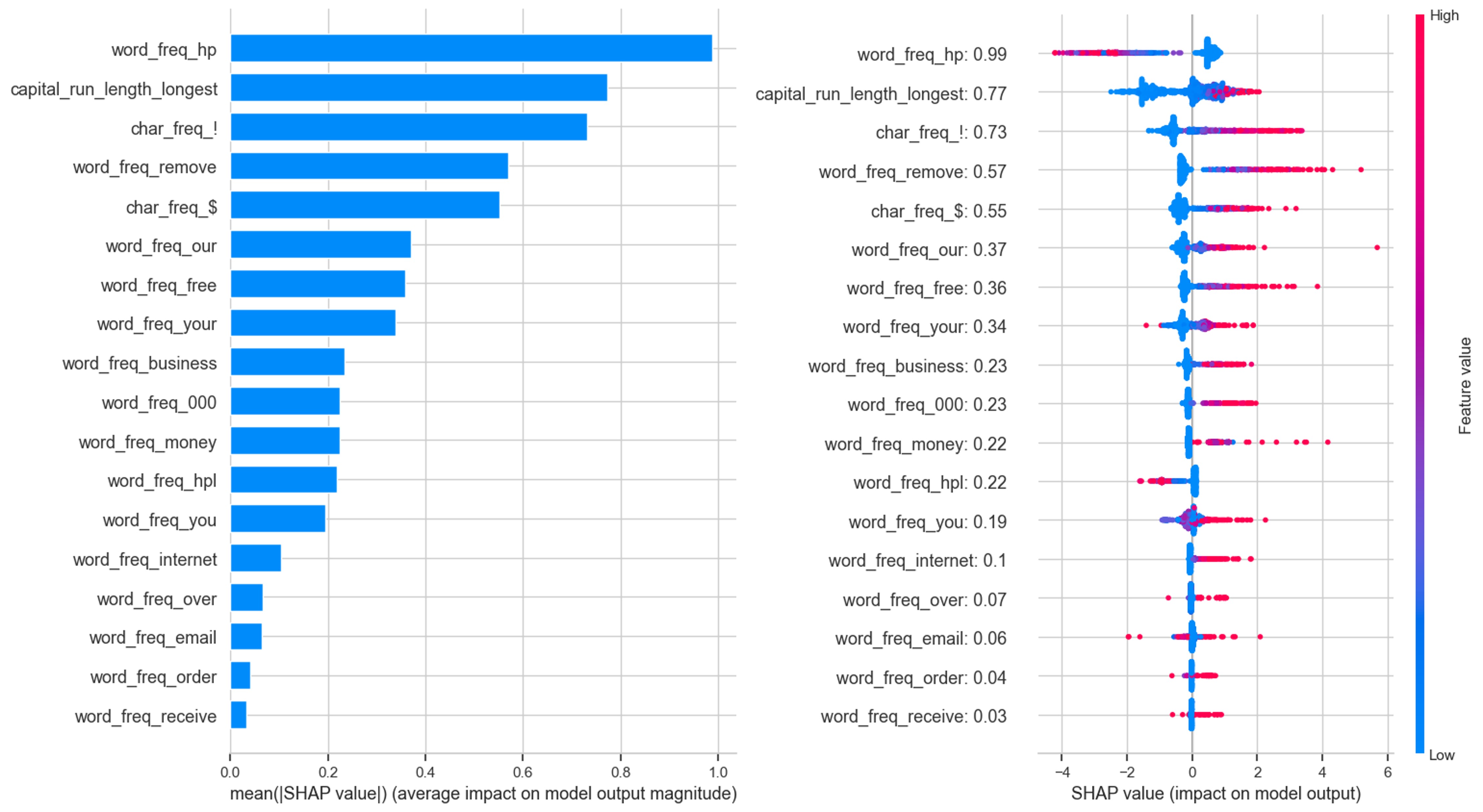
The plot above shows the absolute SHAP value which tells us how much a single feature affected the prediction.The frequency of the word 'hp', the length of sequential capital letters and the frequency of the '!' character were the top 3 factors for this observation.
From this plot, red values indicate a positive contribution (spam) while blue values indicate a negative contribution (not spam) to the prediction. From here we can see the following:
- A high positive contribution is obtained for word_freq_hp when the SHAP values are negative.
- A high negative contribution is obtained for capital_run_length_longest when the SHAP values are negative
- A high positive contribution is obtained for char_freq_! when the SHAP values are positive
Applying the Model to the Entire Dataset
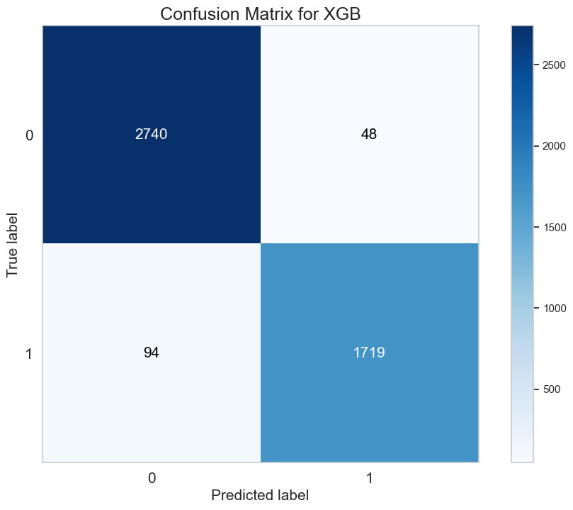
Let's now see how the model performs over the entire dataset.
The confusion matrix of the model applied over the entire dataset (4601 emails) is shown below. The XGB resulted in 48 false positives and 94 false negatives. It also has 2740 true positives and 1719 true negatives. This represents a 1% error in classfying a non-spam email as spam, a 2% error in classifying a spam email as non-spam, and an overall 97% classification accuracy which is pretty good!
The interactive visualization below shows the SHAP values for ALL the emails in the dataset which allows you too see how the model decided to classify each email as spam or not spam.
Conclusions
The spambase dataset was used to train a machine learning model capable of classifying emails as spam with 97% accuracy using the XGBoost Classifier. The model was optimized to have an AUC of 0.91, a sensitivity of 0.92, and a specificity of 0.94.
Thanks for reading!